Slab model
The purpose of dustpylib.radtrans.slab is to implement a simple, plane-parallel slab solution for protoplanetary disks and to compute those based on files from DustPy simulations.
In this notebook we are going to produce a radio images from the planetary gaps example in the DustPy documentation. This repository contains a reduced DustPy output file of the final snapshot of the example model only containing the fields that are required to produce the RADMC-3D model. We will use the same to compute such an image with the slab model for comparison.
All quantities are in CGS units.
In the first step we need to load the DustPy data file using the hdf5writer for this.
[1]:
from pathlib import Path

import numpy as np
import matplotlib.pyplot as plt

from dustpy import hdf5writer
import dustpy.constants as c
from dustpylib.radtrans import radmc3d
Read in the dustpy snapshot
[2]:
writer = hdf5writer()
writer.datadir = "example_planetary_gaps"
data = writer.read.output(21)
Creating a RADMC-3D model for comparison
To compare the results of the slab model with a “ground truth” result use RADMC-3D. The following cells are taken from the radmc3d.ipynb notebook but only creates the setup and computes the radio image.
[3]:
plt.rcParams["figure.dpi"] = 150.
rt = radmc3d.Model(data)
rt.phii_grid = np.array([0., 2.*np.pi])
rt.ai_grid = np.geomspace(rt.a_dust_.min(), 1., 17)
rt.radmc3d_options["nphot"] = 500_000
rt.radmc3d_options["nphot_scat"] = 500_000
rt.radmc3d_options["nphot_spec"] = 10_000
rt.radmc3d_options["mc_scat_maxtauabs"] = 5.
rt.radmc3d_options["dust_2daniso_nphi"] = 60
rt.datadir = "radmc3d"
rt.write_files()
img_name = "radmc3d/image_radio.out"
Writing radmc3d/radmc3d.inp.....done.
Writing radmc3d/stars.inp.....done.
Writing radmc3d/wavelength_micron.inp.....done.
Writing radmc3d/amr_grid.inp.....done.
Writing radmc3d/dust_density.inp.....done.
Writing radmc3d/dust_temperature.dat.....done.
Writing radmc3d/dustopac.inp.....done.

Computing opacities...
Using dsharp_opac. Please cite Birnstiel et al. (2018).
Using DSHARP mix. Please cite Birnstiel et al. (2018).
Please cite Warren & Brandt (2008) when using these optical constants
Please cite Draine 2003 when using these optical constants
Reading opacities from troilitek
Please cite Henning & Stognienko (1996) when using these optical constants
Reading opacities from organicsk
Please cite Henning & Stognienko (1996) when using these optical constants
| material                            | volume fractions | mass fractions |
|-------------------------------------|------------------|----------------|
| Water Ice (Warren & Brandt 2008)    | 0.3642           | 0.2            |
| Astronomical Silicates (Draine 2003)| 0.167            | 0.329          |
| Troilite (Henning)                  | 0.02578          | 0.07434        |
| Organics (Henning)                  | 0.443            | 0.3966         |
Mie ... Done!

Writing radmc3d/dustkapscatmat_00.inp.....done.
Writing radmc3d/dustkapscatmat_01.inp.....
/Users/birnstiel/pixi/base/.pixi/envs/dustpy/lib/python3.12/site-packages/dsharp_opac/dsharp_opac.py:2885: RuntimeWarning: invalid value encountered in scalar divide
  g[grain, i] = -2 * np.pi * \
done.
Writing radmc3d/dustkapscatmat_02.inp.....done.
Writing radmc3d/dustkapscatmat_03.inp.....done.
Writing radmc3d/dustkapscatmat_04.inp.....done.
Writing radmc3d/dustkapscatmat_05.inp.....done.
Writing radmc3d/dustkapscatmat_06.inp.....done.
Writing radmc3d/dustkapscatmat_07.inp.....done.
Writing radmc3d/dustkapscatmat_08.inp.....done.
Writing radmc3d/dustkapscatmat_09.inp.....done.
Writing radmc3d/dustkapscatmat_10.inp.....done.
Writing radmc3d/dustkapscatmat_11.inp.....done.
Writing radmc3d/dustkapscatmat_12.inp.....done.
Writing radmc3d/dustkapscatmat_13.inp.....done.
Writing radmc3d/dustkapscatmat_14.inp.....done.
Writing radmc3d/dustkapscatmat_15.inp.....done.

Writing radmc3d/metadata.npz.....done.
Run these to compute/rename the image file if you want to re-recreate it
!cd {rt.datadir} && radmc3d image lambda 1300 sizeau 100 npixx 512 npixy 512 setthreads 8
!mv  {Path(rt.datadir) / 'image.out'} {img_name}
[4]:
image_radio = radmc3d.read_image(img_name)
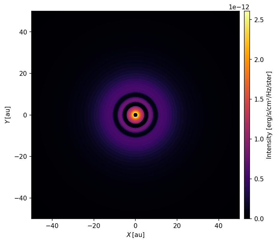
Plot the RADMC3D Image
[5]:
x, y = image_radio["x"] / c.au, image_radio["y"] / c.au

fig, ax = plt.subplots(figsize=(6, 6))
ax.set_aspect(1)
pcm = ax.pcolormesh(
    x, y, image_radio["I"][..., 0].T,
    cmap="inferno", vmin=0, vmax=image_radio['I'].max())
ax.set(xlabel=r"$X\,\left[\mathrm{au}\right]$", ylabel=r"$Y\,\left[\mathrm{au}\right]$")

pos = ax.get_position()
cbar = fig.colorbar(pcm, cax=fig.add_axes([1.02 * pos.x1, pos.y0, 0.02, pos.y1 - pos.y0]))
cbar.set_label(r"Intensity [erg/s/cm²/Hz/ster]")
Compute the radial profile
[6]:
from scipy.stats import binned_statistic
X, Y = np.meshgrid(image_radio['x'], image_radio['y'], indexing='ij')
R = np.sqrt(X**2 + Y**2)
# define the bins
ri_bins = np.geomspace(np.abs(R).min(), R.max(), 100)
r_bins = 0.5 * (ri_bins[1:] + ri_bins[:-1])
# get the averaged intensity profile
profile = binned_statistic(R.ravel(), image_radio['I'][...,0].ravel(), bins=ri_bins).statistic
Use the Slab Model
[7]:
from dustpylib.radtrans import slab

if rt.opacity == 'birnstiel2018':
    opacity_file = 'default_opacities_smooth.npz'
else:
    opacity_file = None

opac = slab.Opacity(opacity_file)
lam = image_radio['lambda']

obs = slab.get_all_observables(data, opac, lam)
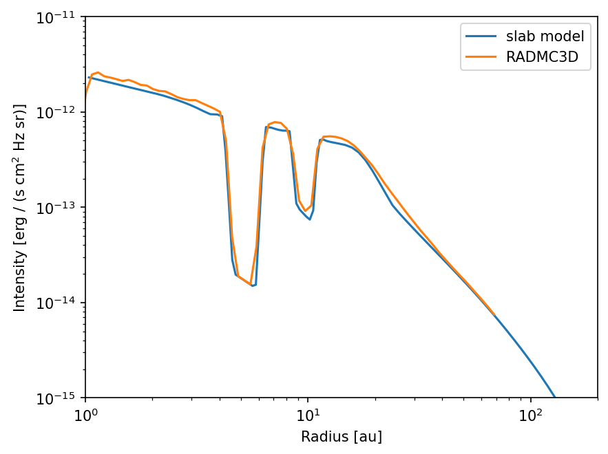
[8]:
f, ax = plt.subplots()
ax.loglog(data.grid.r / c.au, obs.I_nu[0, :] * slab.slab.jy_sas, label='slab model')
ax.loglog(r_bins / c.au, profile, label='RADMC3D')
ax.set(ylim=[1e-15, 1e-11], xlim=[1, 200], xlabel='Radius [au]', ylabel='Intensity [erg / (s cm$^2$ Hz sr)]')
ax.legend();