RADMC-3D

RADMC-3D is a Monte Carlo Radiative Transfer software package for astrophysics. The purpose of dustpylib.radtrans.radmc3d is to produce RADMC-3D input files from DustPy simulations.

For details on the usage of RADMC-3D please have a look at the RADMC-3D documentation.

This module creates axisymmetric disk models where the dust particles are vertically distributed according their scale heights. Dust opacities are created using the dsharp_opac package (Birnstiel et al., 2018).

The intent of this module is not to provide a fully customizable interface to RADMC-3D, but rather to provide a minimum working setup, that can be further customized manually.

In this notebook we are going to produce RADMC-3D images from the planetary gaps example in the DustPy documentation. This repository contains a reduced DustPy output file of the final snapshot of the example model only containing the fields that are required to produce the RADMC-3D model. The example contains the default DustPy setup with Jupiter and Saturn added at their current locations.

This notebook only demonstrates the usage of the DustPyLib module. RADMC-3D has to be installed and executed manually.

All quantities are in CGS units.

In the first step we need to load the DustPy data file using the hdf5writer for this.

from dustpy import hdf5writer

writer = hdf5writer()
writer.datadir = "example_planetary_gaps"

data = writer.read.output(21)

Creating the RADMC-3D model

We can now use dustpylib.radtrans.radmc3d to produce the model intput files. The Model class accepts either a DustPy.Simulation object directly or a namespace as returned by the Writer.read.output() method.

from dustpylib.radtrans import radmc3d

rt = radmc3d.Model(data)

The Model object contains several attributes, that can be modified, where by definition attibutes with trailing _ are imported from the DustPy model, while the ones without are used in the RADMC-3D model, e.g. the grid.

By default the outermost grid cell of the DustPy simulation will be ignored. By default the outer boundary condition of the gas is the floor value. This leads to very large Stokes numbers of the particles and therefore to very small dust scale heights and very large midplane dust densities. This can lead to unwanted features when the data is interpolated onto the RADMC3D grid. To use the last radial grid cell nevertheless, set the ignore_last keyword argument to False, for example rt = radmc3d.Model(data, ignore_last=False).

The RADMC-3D model parameters are chosen reasonably, but can be customized if needed.

Some scattering modes of RADMC-3D require both hemispheres (\(\theta\)-grid) of the disk and an azimuthal grid (\(\varphi\)-grid), while other modes can work with a single hemisphere or a single azimuthal cell. The module will by default create both hemispheres (\(\theta\)-grid from \(0\) to \(\pi\) with \(256\) grid cells) and a coarse azimuthal grid (\(\varphi\)-grid from \(0\) to \(2\pi\) with \(16\) grid cells).

In this notebook we are going to use scattering mode 5, which requires both hemispheres but does not require an azimuthal grid. We can therefore turn off the azimuthal grid by only providing two grid cell interfaces. You can customize all grids by setting the grid cell interfaces. Do not set the grid cell centers directly. This will happen automatically.

import numpy as np

rt.phii_grid = np.array([0., 2.*np.pi])

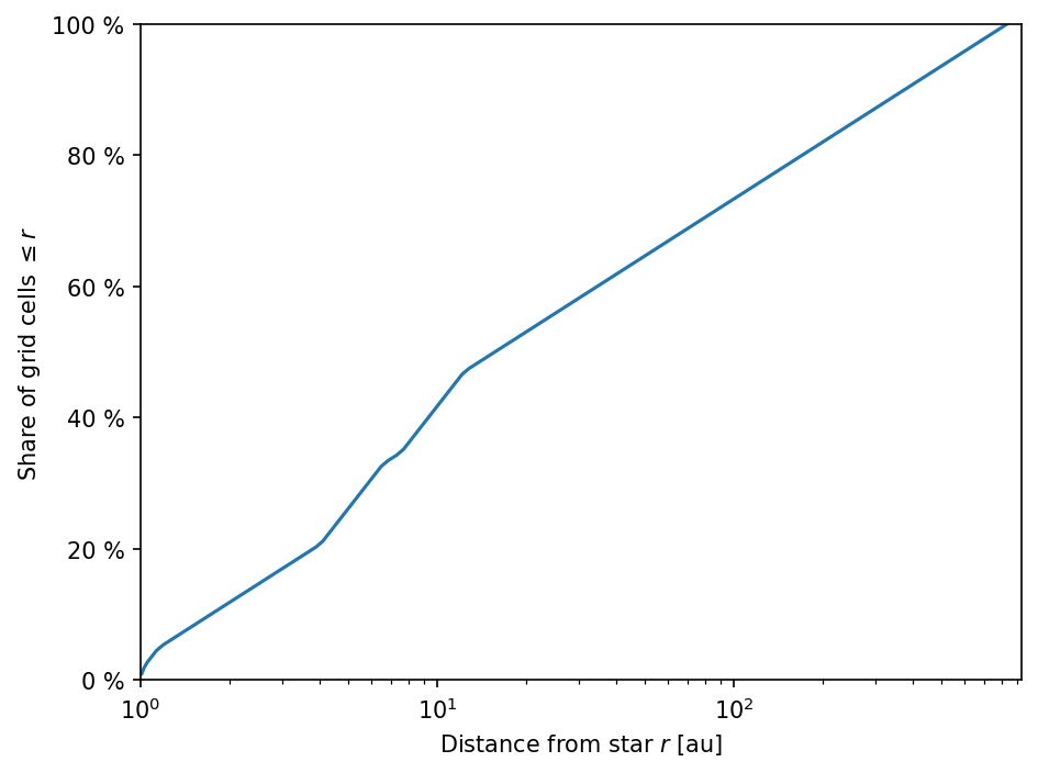
The inner edge of the disk is directly illuminated by the star and typically the densest part of the disk and therefore optically thick. Because of this the radial grid of the RADMC-3D setup is slightly refined in the inner part.

Note, that in this specific example the DustPy grid has been refined at the location of the planets, which will then be also the case in the default RADMC-3D model setup. A steeper slope means a finer radial grid.

import dustpy.constants as c
import matplotlib.pyplot as plt

plt.rcParams["figure.dpi"] = 150.

fig, ax = plt.subplots()
Ncells = rt.rc_grid.shape[0]
ax.semilogx(rt.rc_grid/c.au, np.linspace(1., 101., Ncells))
ax.set_xlabel("Distance from star $r$ [au]")
ax.set_ylabel("Share of grid cells $\leq r$")
ax.set_xlim(rt.ri_grid[0]/c.au, rt.ri_grid[-1]/c.au)
ax.set_ylim(0., 100.)
ax.set_yticks(ax.get_yticks())
ax.set_yticklabels(["{:.0f} %".format(t) for t in ax.get_yticks()])
fig.tight_layout()

DustPy typically uses more particle species than one would want to use in radiative transfer models for performance reasons. By default this module uses only 16 dust species between the smallest and largest sizes in the DustPy setup. However, as can be seen in the example notebook some of the larger bins are actually empty. It is therefore advisable to inspect the actual particle sizes and adjust the RADMC-3D size grid accordingly.

The largest particle are in the inner disk. We therefore have a look at the innermost DustPy grid cell.

fig, ax = plt.subplots()
ax.loglog(rt.a_dust_[0, :], rt.Sigma_dust_[0, :])
ax.set_xlabel("Particle size [cm]")
ax.set_ylabel(r"$\Sigma_\mathrm{dust}$ [g/cm²]")
ax.set_xlim(rt.a_dust_.min(), rt.a_dust_.max())
ax.set_ylim(1.e-8, 1.e1)
fig.tight_layout()

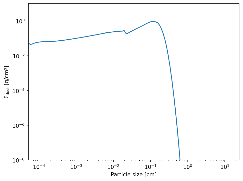
We therefore re-define the particle size grid of the RADMC-3D model with a maximum particle size of 1 cm. Note, that we have to set the interfaces of the size bins and there are 17 grid cell interfaces needed for 16 particle species.

The hundreds of DustPy particle species will then be re-binned onto this grid while conserving mass.

rt.ai_grid = np.geomspace(rt.a_dust_.min(), 1., 17)

The central particle size of a size bin is automatically calculated.

rt.ac_grid

array([7.45574916e-05, 1.38067479e-04, 2.55676905e-04, 4.73469062e-04,
       8.76782175e-04, 1.62364776e-03, 3.00671264e-03, 5.56790773e-03,
       1.03107946e-02, 1.90937944e-02, 3.53583790e-02, 6.54775548e-02,
       1.21253018e-01, 2.24539455e-01, 4.15807933e-01, 7.70003814e-01])

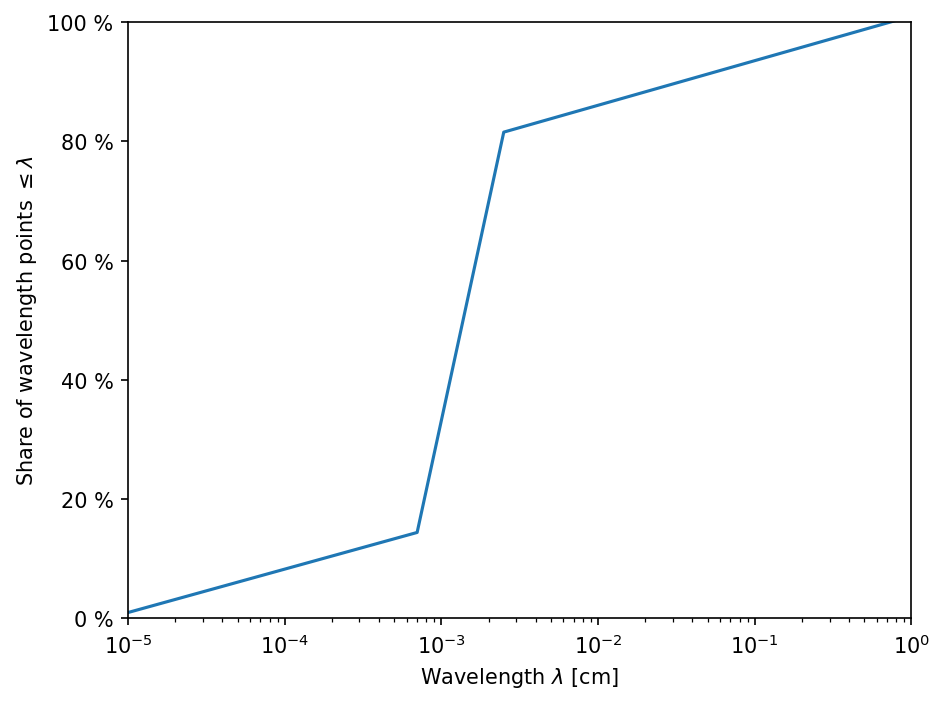
The default wavelength grid will cover wavelengths from \(0.1\,\mu\mathrm{m}\) to \(1\,\mathrm{cm}\) with a refinement around the \(10\,\mu\mathrm{m}\) dust feature. The wavelength grid needs to cover those wavelengths at which the star mostly radiates and those wavelengths at which the dust particles predominantly cool. For hot stars (\(\gtrsim 10\,000\,\mathrm{K}\)) the wavelengths grid has to be extended to smaller wavelengths. If the wavelengths are too small, however, computation of the opacities can fail, if the wavelengths are out of range of the optical constants used to calculate the opacities.

Note, that RADMC-3D uses microns for wavelengths. This module, however, uses exclusively CGS units and converts the quantities internally, if needed.

fig, ax = plt.subplots()
Ncells = rt.lam_grid.shape[0]
ax.semilogx(rt.lam_grid, np.linspace(1., 101., Ncells))
ax.set_xlabel("Wavelength $\lambda$ [cm]")
ax.set_ylabel("Share of wavelength points $\leq \lambda$")
ax.set_xlim(rt.lam_grid[0], rt.lam_grid[-1])
ax.set_ylim(0., 100.)
ax.set_yticks(ax.get_yticks())
ax.set_yticklabels(["{:.0f} %".format(t) for t in ax.get_yticks()])
fig.tight_layout()

Additional options for the radmc3d.inp file can be added to the radmc3d_options dictionary.

rt.radmc3d_options

{'modified_random_walk': 1, 'iranfreqmode': 1, 'istar_sphere': 1}

We want to use \(10\,000\,000\) photons for the thermal run, \(1\,000\,000\) photons for the scattering run, and \(10\,000\) for the spectral run.

rt.radmc3d_options["nphot"] = 10_000_000
rt.radmc3d_options["nphot_scat"] = 1_000_000
rt.radmc3d_options["nphot_spec"] = 10_000

The maximum optical depth of absorption at which photons get destroyed is by default \(30\). In this notebook we want to decrease this value to \(5\).

rt.radmc3d_options["mc_scat_maxtauabs"] = 5.

DustPyLib will create opacity files that allow for the most complex scattering mode. In this notebook we want to use the largest possible mode. We therefore do not specify scattering_mode_max.

For the scattering mode we are using here, RADMC-3D internally creates a \(\varphi\)-grid. To speed up the computation we want to reduce the number of grid cells from the default of 360 to 60.

rt.radmc3d_options["dust_2daniso_nphi"] = 60

We want to store the RADMC-3D input files in the following directory

rt.datadir = "radmc3d"

To compute the dust opacities DustPyLib uses the dsharp_opac package. Two different opacity models can be used: The DSHARP opacities (Model.opacity="birnstiel2018", Birnstiel et al., 2018, default) or the Ricci opacities (Model.opacity="ricci2010", Ricci et al., 2010). Please cite all references that are printed during the computations.

The Model.write_files() has additional options. If you do not want to compute opacities, you can set writeopacities=False. If you want to use smoothed opacities, use smooth_opacities=True. In that case the opacities are not calculated for a singular particle size per bin, but for several sizes and then averaged. Note, that this will take significantly longer.

This module furthermore writes the file metadata.npz, which is not needed for the RADMC-3D model setup, but contains additional data that may be useful for postprocessing. In this case the particle sizes.

We can now create the RADMC-3D model files.

rt.write_files()

Writing radmc3d/radmc3d.inp.....done.
Writing radmc3d/stars.inp.....done.
Writing radmc3d/wavelength_micron.inp.....done.
Writing radmc3d/amr_grid.inp.....done.
Writing radmc3d/dust_density.inp.....done.
Writing radmc3d/dust_temperature.dat.....done.
Writing radmc3d/dustopac.inp.....done.

Computing opacities...
Using dsharp_opac. Please cite Birnstiel et al. (2018).
Using DSHARP mix. Please cite Birnstiel et al. (2018).
Please cite Warren & Brandt (2008) when using these optical constants
Please cite Draine 2003 when using these optical constants
Reading opacities from troilitek
Please cite Henning & Stognienko (1996) when using these optical constants
Reading opacities from organicsk
Please cite Henning & Stognienko (1996) when using these optical constants
| material                            | volume fractions | mass fractions |
|-------------------------------------|------------------|----------------|
| Water Ice (Warren & Brandt 2008)    | 0.3642           | 0.2            |
| Astronomical Silicates (Draine 2003)| 0.167            | 0.329          |
| Troilite (Henning)                  | 0.02578          | 0.07434        |
| Organics (Henning)                  | 0.443            | 0.3966         |
Mie ... Done!

/home/stammler/anaconda3/envs/j/lib/python3.11/site-packages/dsharp_opac/dsharp_opac.py:2778: RuntimeWarning: invalid value encountered in scalar divide
  g[grain, i] = -2 * np.pi * np.trapz(zscat[grain, i, :, 0] * mu, x=mu) / k_sca[grain, i]

Writing radmc3d/dustkapscatmat_00.inp.....done.
Writing radmc3d/dustkapscatmat_01.inp.....done.
Writing radmc3d/dustkapscatmat_02.inp.....done.
Writing radmc3d/dustkapscatmat_03.inp.....done.
Writing radmc3d/dustkapscatmat_04.inp.....done.
Writing radmc3d/dustkapscatmat_05.inp.....done.
Writing radmc3d/dustkapscatmat_06.inp.....done.
Writing radmc3d/dustkapscatmat_07.inp.....done.
Writing radmc3d/dustkapscatmat_08.inp.....done.
Writing radmc3d/dustkapscatmat_09.inp.....done.
Writing radmc3d/dustkapscatmat_10.inp.....done.
Writing radmc3d/dustkapscatmat_11.inp.....done.
Writing radmc3d/dustkapscatmat_12.inp.....done.
Writing radmc3d/dustkapscatmat_13.inp.....done.
Writing radmc3d/dustkapscatmat_14.inp.....done.
Writing radmc3d/dustkapscatmat_15.inp.....done.

Writing radmc3d/metadata.npz.....done.

The RADMC-3D model is now ready to go. Of course, all files, especially radmc3d.inp, can be customized manually.

Inspecting the RADMC-3D model

dustpylib.radtrans.radmc3d has a simple method to load the RADMC-3D model files to inspect the setup before executing RADMC-3D. It does only work for models created with DustPyLib due to the assumed symmetries. For more general methods for analyzing models, use radmc3dPy that comes with RADMC-3D.

model = radmc3d.read_model(datadir="radmc3d")

We can now plot the densities and temperatures of the RADMC-3D model.

def plot_model(model, spec=-1):
    """
    Function plots the RADMC-3D model.

    Parameters
    ----------
    model : namespace
        The RADMC-3D model data
    spec : integer, optional, default : -1
        Particle species to be plotted. If -1, the total
        dust densities are plotted.
    """
    width = 6.
    height = width/1.3

    if spec==-1:
        rho = np.maximum(np.hstack((model.rho[:, :1, 0, :].sum(-1), model.rho[:, :, 0, :].sum(-1))), 1.e-100)
        T = np.hstack((model.T[:, :1, :, 0], model.T[:, :, :, 0])).mean(-1)
        a_rho = "total"
        a_T = "$a$ = {:.2e} cm".format(model.grid.a[0])
    else:
        rho = np.maximum(np.hstack((model.rho[:, :1, 0, spec], model.rho[:, :, 0, spec])), 1.e-100)
        T = np.hstack((model.T[:, :1, :, spec], model.T[:, :, :, spec])).mean(-1)
        a_rho = "$a$ = {:.2e} cm".format(model.grid.a[spec])
        a_T = "$a$ = {:.2e} cm".format(model.grid.a[spec])

    rho = np.hstack((rho, np.flip(rho[:, 1:, ...], 1)))
    T = np.hstack((T, np.flip(T[:, 1:, ...], 1)))

    theta = np.hstack((model.grid.theta[0]-(model.grid.theta[1]-model.grid.theta[0]), model.grid.theta))
    theta = np.hstack((theta, theta[1:]+np.pi))
    lev_rho_max = np.ceil(np.log10(rho.max()))
    levels_rho = np.arange(lev_rho_max-6, lev_rho_max+1, 1.)

    fig, ax = plt.subplots(ncols=2, figsize=(2*width, height), subplot_kw={"projection": "polar"})

    p0 = ax[0].contourf(theta, model.grid.r/c.au, np.log10(rho), levels=levels_rho, extend="both", cmap="viridis")
    ax[0].contourf(-theta, model.grid.r/c.au, np.log10(rho), levels=levels_rho, extend="both", cmap="viridis")
    ax[0].set_theta_zero_location("N")
    ax[0].set_rlim(0)
    ax[0].set_rscale("symlog")
    ax[0].set_rgrids([1., 10., 100.], angle=-45)
    ax[0].tick_params(axis='y', colors='white')
    ax[0].set_xticks([])
    ax[0].plot(0., 0., "*", color="C3", markeredgewidth=0, markersize=12)
    cbar0 = plt.colorbar(p0)
    cbar0.set_ticks(cbar0.get_ticks())
    cbar0.set_ticklabels(["$10^{{{:d}}}$".format(int(t)) for t in cbar0.get_ticks()])
    cbar0.set_label(r"$\rho_\mathrm{dust}$ [g/cm³]")
    ax[0].set_title("Dust density, {}".format(a_rho))

    p1 = ax[1].contourf(theta, model.grid.r/c.au, T, extend="both", cmap="coolwarm")
    ax[1].contourf(-theta, model.grid.r/c.au, T, extend="both", cmap="coolwarm")
    ax[1].set_theta_zero_location("N")
    ax[1].set_rlim(0)
    ax[1].set_rscale("symlog")
    ax[1].set_rgrids([1., 10., 100.], angle=-45)
    ax[1].tick_params(axis='y', colors='black')
    ax[1].set_xticks([])
    ax[1].plot(0., 0., "*", color="C3", markeredgewidth=0, markersize=12)
    cbar1 = plt.colorbar(p1)
    cbar1.set_ticks(cbar1.get_ticks())
    cbar1.set_label(r"$T$ [K]")
    ax[1].set_title("Dust temperature, {}".format(a_T))

    fig.tight_layout()

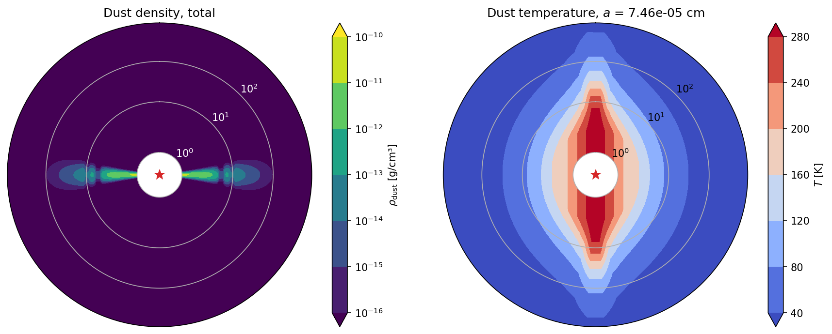
This DustPyLib modules creates the dust_temperature.dat file, which should be self-consistently calculated with RADMC-3D.

However, DustPyLib stores the temperatures that DustPy used during the simulation and assumes a vertically isothermal temperature and, furthermore, that all dust species have the same temperature as the gas. Note, the temperatures in the plot do not look vertically isothermal due to a combination of the coarse \(\theta\)-grid and the logarithmic r-axis.

We can plot the total dust densities with spec=-1.

plot_model(model, spec=-1)

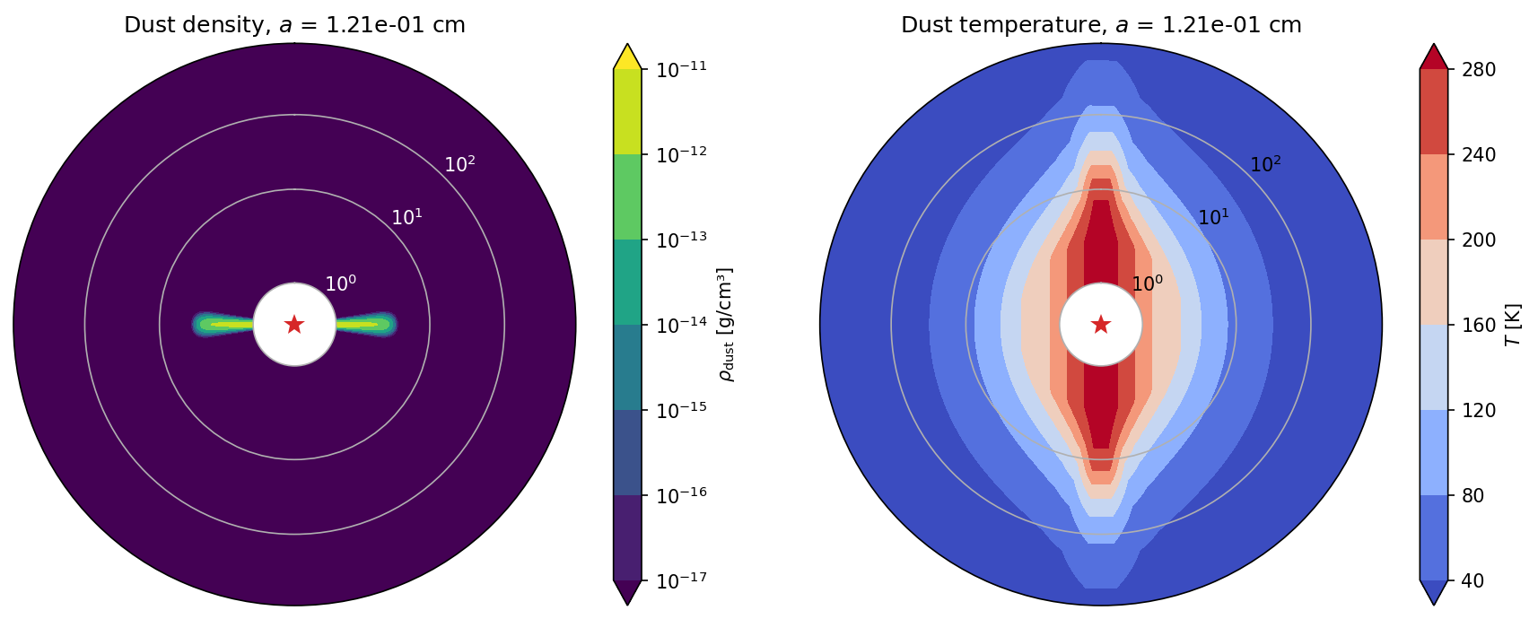
Or plot specific dust species.

plot_model(model, spec=12)

Thermal Monte Carlo run

In the first step we run the thermal Monte Carlo process in which the dust temperatures are computed. This can be done by executing the following command in the directory containing the RADMC-3D input files.

radmc3d mctherm

This will overwrite the DustPy temperatures in the dust_temperature.dat file with the temperatures self-consistently computed by RADMC-3D. This has been done for this notebook already and the temperature file can be simply copied.

import shutil

shutil.copy("radmc3d/dust_temperature_mctherm.dat", "radmc3d/dust_temperature.dat")

'radmc3d/dust_temperature.dat'

To plot the new temperatures we have to read the model files again.

model_mc = radmc3d.read_model(datadir="radmc3d")

plot_model(model_mc, spec=-1)

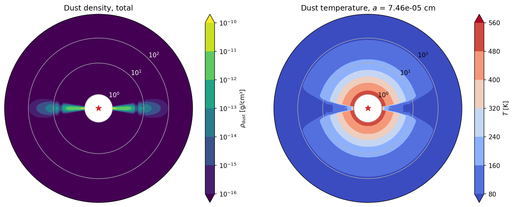
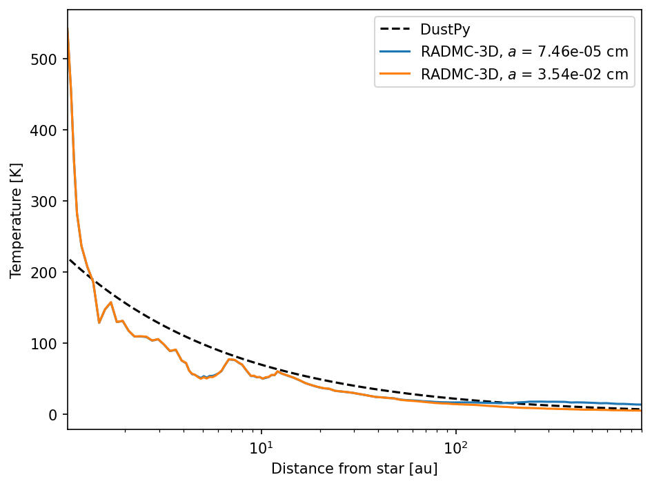
We can now compare the midplane temperature that DustPy uses with the temperatures that RADMC-3D calculated. We are taking the mean temperature in azimuthal direction (only one grid cell in this setup) and the mean temperature of 5 grid cells above and below the midplane to reduce the Monte Carlo noise.

Note that the temperature at the inner edge of the disk is significantly increased in the RADMC-3D model, since it it directly illuminated by the star. DustPy, on the other hand, does not assume that the disk ends at the inner edge of the radial grid.

imid = int(model_mc.grid.theta.shape[0]/2)-1
irange = 5
fig, ax = plt.subplots()
ax.plot(data.grid.r/c.au, data.gas.T, "--", label="DustPy", c="black")
ax.plot(model_mc.grid.r/c.au, model_mc.T[:, imid-irange:imid+irange, :, 0].mean((-2, -1)), label="RADMC-3D, $a$ = {:.2e} cm".format(rt.ac_grid[0]))
ax.plot(model_mc.grid.r/c.au, model_mc.T[:, imid-irange:imid+irange, :, 10].mean((-2, -1)), label="RADMC-3D, $a$ = {:.2e} cm".format(rt.ac_grid[10]))
ax.set_xscale("log")
ax.set_xlim(model_mc.grid.r[0]/c.au, model_mc.grid.r[-1]/c.au)
ax.set_xlabel("Distance from star [au]")
ax.set_ylabel("Temperature [K]")
ax.legend()
fig.tight_layout()

Radio images

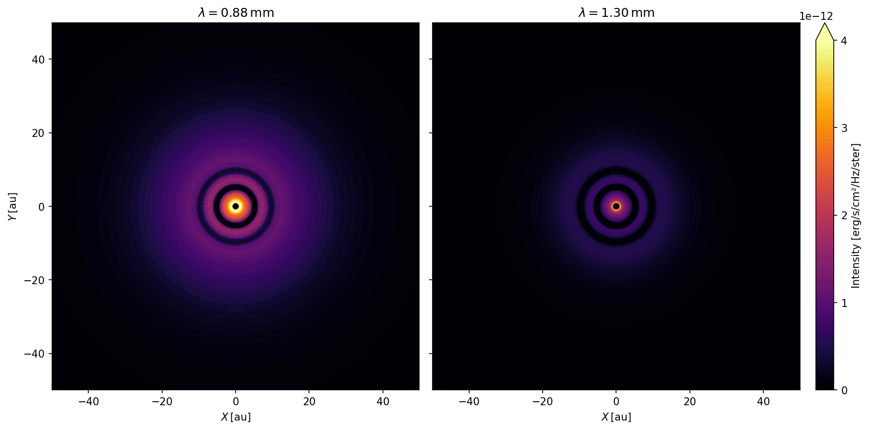
We can now use RADMC-3D to create millimeter observations as obtained for example with ALMA.

We are going to create two images: one at \(\lambda = 0.88\,\mathrm{mm}\) (Band 7) and one at \(\lambda = 1.3\,\mathrm{mm}\) (Band 6). Furthermore, we are focussing on the inner \(50\,\mathrm{au}\) of the disk with 512 pixels in each direction. This can be done with the following RADMC-3D command:

radmc3d image lambdarange 880 1300 nlam 2 sizeau 100 npixx 512 npixy 512

Afterwards we rename the image file with:

mv image.out image_radio.out

For more details have a look at the imaging chapter of the RADMC-3D documentation.

We can now use DustPyLib to load the image with the following helper function, which returns a dictionary.

image_radio = radmc3d.read_image("radmc3d/image_radio.out")

width = 6.
height = width
x, y = image_radio["x"]/c.au, image_radio["y"]/c.au
Imax = 0.5*image_radio["I"].max()
mag = np.floor(np.log10(Imax))
logmax = np.ceil(Imax * 10**(-mag))
levels = np.linspace(0., logmax, 100) * 10**mag
ticks = np.arange(int(logmax)+1) * 10**mag
fig, ax = plt.subplots(ncols=2, figsize=(2*width, height), sharey=True)
ax[0].set_aspect(1)
ax[0].contourf(x, y, image_radio["I"][..., 0].T, cmap="inferno", levels=levels, extend="max")
ax[0].set_title("$\lambda = {:.2f}\,\mathrm{{mm}}$".format(image_radio["lambda"][0]*10.))
ax[0].set_xlabel(r"$X\,\left[\mathrm{au}\right]$")
ax[0].set_ylabel(r"$Y\,\left[\mathrm{au}\right]$")
ax[1].set_aspect(1)
p = ax[1].contourf(x, y, image_radio["I"][..., 1].T, cmap="inferno", levels=levels, extend="max")
ax[1].set_title("$\lambda = {:.2f}\,\mathrm{{mm}}$".format(image_radio["lambda"][1]*10.))
ax[1].set_xlabel(r"$X\,\left[\mathrm{au}\right]$")
fig.tight_layout()
fig.subplots_adjust(right=0.9)
pos01 = ax[1].get_position()
cb_ax = fig.add_axes([1.02*pos01.x1, pos01.y0, 0.02, pos01.y1-pos01.y0])
cbar = fig.colorbar(p, cax=cb_ax)
cbar.set_ticks(ticks)
cbar.set_label(r"Intensity [erg/s/cm²/Hz/ster]")

Note that RADMC-3D comes with a Python support package to create .fits files from images which can the be further processed by CASA.

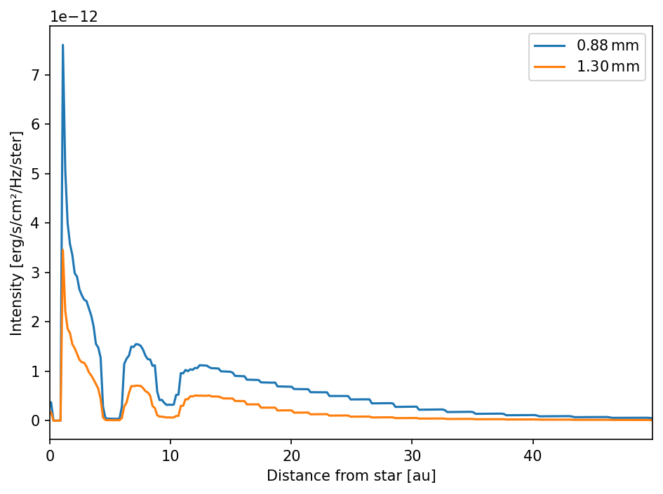
We can additionally plot the radial intensity profiles.

x = image_radio["x"]/c.au
Nx = x.shape[0]
fig, ax = plt.subplots()
ax.plot(x, image_radio["I"][:, int(Nx/2), 0], label="${:.2f}\,\mathrm{{mm}}$".format(image_radio["lambda"][0]*10.))
ax.plot(x, image_radio["I"][:, int(Nx/2), 1], label="${:.2f}\,\mathrm{{mm}}$".format(image_radio["lambda"][1]*10.))
ax.set_xlim(0., x.max())
ax.set_xlabel("Distance from star [au]")
ax.set_ylabel(r"Intensity [erg/s/cm²/Hz/ster]")
ax.legend()
fig.tight_layout()

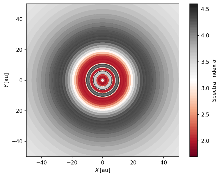
Spectral index maps

Since we created images at two different wavelengths we can create spectral index maps.

alpha = -np.log10(image_radio["I"][..., 0]/image_radio["I"][..., 1]) / np.log10(image_radio["lambda"][0]/image_radio["lambda"][1])

x, y = image_radio["x"], image_radio["y"]
levels = np.linspace(1.7, 4.6, 100)
ticks = np.arange(2.0, 4.6, 0.5)
fig, ax = plt.subplots()
ax.set_aspect(1)
p = ax.contourf(x/c.au, y/c.au, alpha.T, cmap="RdGy", levels=levels)
ax.set_xlabel(r"$X\,\left[\mathrm{au}\right]$")
ax.set_ylabel(r"$Y\,\left[\mathrm{au}\right]$")
cbar = plt.colorbar(p)
cbar.set_ticks(ticks)
cbar.set_label(r"Spectral index $\alpha$")
ax.set_xlim(-50., 50)
ax.set_ylim(-50., 50)
fig.tight_layout()

Polarization maps

To create images with polarization information we have to append the stokes flag to the RADMC-3D command. We only do this here for a single wavelength

radmc3d image lambda 880 sizeau 100 npixx 512 npixy 512 stokes

and rename the image file

mv image.out image_polarization.out

image_polarization = radmc3d.read_image("radmc3d/image_polarization.out")

Now we can calculate the polarization fraction.

I, Q, U = image_polarization["I"], image_polarization["Q"], image_polarization["U"]
P = np.sqrt(Q**2+U**2)/I

Then we have to convert the Stokes-\(Q\) and Stokes-\(U\) into the \(\left(x,y\right)\)-directions of the electric fields. Details on this can be found int the RADMC-3D documentation.

chi = 0.5 * np.arctan2(U, Q)
Ex = np.cos(chi)
Ey = np.sin(chi)

skip = 5
x, y = image_polarization["x"]/c.au, image_polarization["y"]/c.au
levels = np.linspace(0., 0.05, 100)
ticks = np.arange(0., 0.06, 0.01)
fig, ax = plt.subplots()
ax.set_aspect(1)
p = ax.contourf(x, y, P[..., 0].T, cmap="Blues", levels=levels, extend="max")
ax.quiver(x[::skip], y[::skip], Ex[::skip, ::skip, 0], Ey[::skip, ::skip, 0], pivot="mid", headwidth=0, headlength=0, headaxislength=0, color="black", scale=75)
ax.set_xlabel(r"$X\,\left[\mathrm{au}\right]$")
ax.set_ylabel(r"$Y\,\left[\mathrm{au}\right]$")
cbar = plt.colorbar(p)
cbar.set_ticks(ticks)
cbar.set_ticklabels(["{:.0f}%".format(t*100.) for t in cbar.get_ticks()])
cbar.set_label("Polarization fraction")
ax.set_xlim(-20, 20)
ax.set_ylim(-20, 20)
fig.tight_layout()

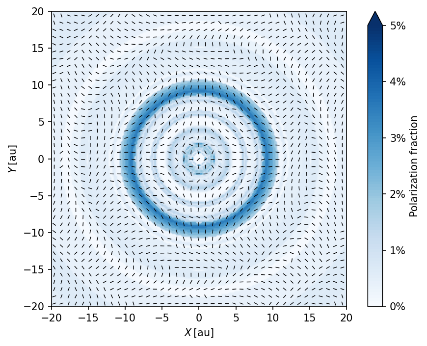
For more information on this polarization pattern, please have a look at Kataoka et al. (2015).

Optical light images

While images at radio wavelengths typically trace the disk midplane, images at optical wavelengths, such as taken with SPHERE at the VLT are heavily affected by scattering at the disk surface.

The approach is identical to the radio images. However, we additionally incline the disk and use a larger field of view to give a better impression of the three-dimensional structure of the disk. We are taking an image at \(\lambda=1.6\,\mu\mathrm{m}\) with the following command

radmc3d image lambda 1.6 sizeau 400 npixx 512 npixy 512 incl 50 posang 53

and rename the image file

mv image.out image_optical.out

image_optical = radmc3d.read_image("radmc3d/image_optical.out")

x, y = image_optical["x"]/c.au, image_optical["y"]/c.au
I = image_optical["I"]
Imax = image_optical["I"].max()
levmax = np.log10(Imax)-2
levels = np.linspace(levmax-6, levmax, 100)
fig, ax = plt.subplots()
ax.set_aspect(1)
ax.contourf(x, y, np.log10(I[..., 0].T), cmap="gist_heat", levels=levels, extend="both")
ax.set_xlabel(r"$X\,\left[\mathrm{au}\right]$")
ax.set_ylabel(r"$Y\,\left[\mathrm{au}\right]$")
ax_ins = ax.inset_axes([0.03, 0.67, 0.32, 0.30])
ax_ins.contourf(x, y, np.log10(I[..., 0].T), cmap="gist_heat", levels=levels, extend="both")
ax_ins.set_xlim(-15, 15)
ax_ins.set_ylim(-15, 15)
ax_ins.xaxis.set_tick_params(labelbottom=False)
ax_ins.yaxis.set_tick_params(labelleft=False)
ax_ins.spines[["top", "left", "bottom", "right"]].set_color("white")
ax.indicate_inset_zoom(ax_ins, edgecolor="white")
fig.tight_layout()

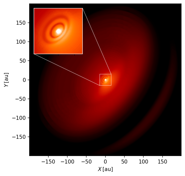
The gaps created by the planets are barely visible in the inner part of the disk in this unconvolved image. Furthermore, we can see the dark midplane at the edge of the disk and some light scattered from the backside of the disk.

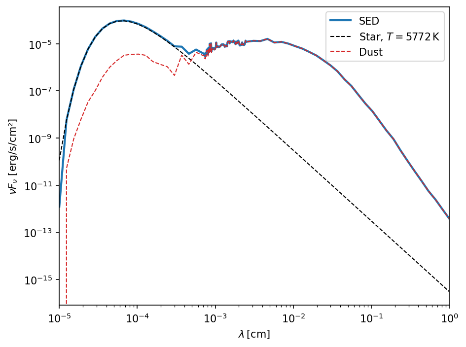
Spectral energy distribution

To create spectra we can use the following command

radmc3d sed

This will create an SED at every wavelength point of the RADMC-3D model. This will take a while, since it is creating an image at every wavelength point.

RADMC-3D will return an SED from a distance of \(1\,\mathrm{pc}\).

spectrum = radmc3d.read_spectrum("radmc3d/spectrum.out")

from astropy.modeling.models import BlackBody
import astropy.constants as ac
import astropy.units as u

lam, F = spectrum["lambda"], spectrum["flux"]
nu = ac.c/(lam*u.cm)
bb = BlackBody(temperature=rt.T_star_*u.K)
conv = (np.pi * ((rt.R_star_*u.cm)/(1.*u.pc))**2.).cgs.value
star = nu.cgs.value*bb(lam*u.cm)*conv
dust = nu.cgs.value*F-star.cgs.value
fig, ax = plt.subplots()
ax.plot(lam, nu.cgs.value*F, label="SED", lw=2)
ax.plot(lam, star, c="black", lw=1, ls="--", label="Star, $T={:.0f}\,\mathrm{{K}}$".format(rt.T_star_))
ax.plot(lam, dust, c="C3", lw=1, ls="--", label="Dust")
ax.set_xscale("log")
ax.set_yscale("log")
ax.set_xlim(lam[0], lam[-1])
ax.set_xlabel(r"$\lambda\,\left[\mathrm{cm}\right]$")
ax.set_ylabel(r"$\nu F_\nu$ [erg/s/cm²]")
ax.legend()
fig.tight_layout()